ComSeg tutorial
ComSeg is an algorithm to perform cell segmentation from RNA point clouds (single cell spatial RNA profiling) from FISH based spatial transcriptomic data. It takes as input a folder of CSV file containing the spots coordiantes of each images and a folder of nucleus segmentation masks for each image. If nucleus segmentation is not available, cell centroids are enough to apply ComSeg.
This tutorial is organized as follow:
Dataset initialization
Create a graph of RNA molecule nodes and apply graph patitioning
In situ clustering
final RNA-nuclei association
[ ]:
[1]:
#### HYPERPARAMETER ####
MEAN_CELL_DIAMETER = 15  # in micrometer
MAX_CELL_RADIUS = 15  # in micrometer
#########################
1) dataset initialization
The first step is to create a comseg-dataset. This object will preprocess the spot coordinates of each images from csv file, add optional prior knowledge and compute the co-expression correlation at the dataset scale.
You need a folder with your spots coordiantes in pixel csv files, with the naming convention {image_name}.csv
You need a folder with you prior segmentation files, with the naming convention {image_name}.tiff
Download the test data for this tutorail at https://cloud.minesparis.psl.eu/index.php/s/zkEfL3fdZyteoXl
[2]:
import pandas as pd
import matplotlib
import comseg
import numpy as np
import random
import tifffile
import importlib
from comseg import dataset as ds
import scanpy
%matplotlib inline
import importlib
#importlib.reload(ds)
/home/tom/.local/lib/python3.8/site-packages/geopandas/_compat.py:124: UserWarning: The Shapely GEOS version (3.11.4-CAPI-1.17.4) is incompatible with the GEOS version PyGEOS was compiled with (3.10.4-CAPI-1.16.2). Conversions between both will be slow.
  warnings.warn(
[3]:
your_path_to_test_data = "/home/tom/Bureau/test_set_tutorial_comseg"


## path to you .csv spots coordinate folder
path_dataset_folder = your_path_to_test_data + "/dataframes"


##path to your prior segmentation mask
path_to_mask_prior = your_path_to_test_data + "/mask"

## scale / pixel size in um
dico_scale = {"x": 0.103, 'y': 0.103, "z": 0.3}


### create the dataset object
dataset = ds.ComSegDataset(
            path_dataset_folder = path_dataset_folder,
            prior_name = 'in_nucleus',
            path_to_mask_prior =path_to_mask_prior,
            dict_scale={"x": 0.103, 'y': 0.103, "z": 0.3},
            mask_file_extension = ".tiff",
    mean_cell_diameter = MEAN_CELL_DIAMETER
)


### add prior knowledge, here using nucleus segmentation mask
dataset.add_prior_from_mask(
                            overwrite = True,
                            compute_centroid = True # compute cell centroid
                           )
add 07_CtrlNI_Pdgfra-Cy3_Serpine1-Cy5_004
add 07_CtrlNI_Pdgfra-Cy3_Serpine1-Cy5_006
add prior to 07_CtrlNI_Pdgfra-Cy3_Serpine1-Cy5_004
prior added to 07_CtrlNI_Pdgfra-Cy3_Serpine1-Cy5_004 and saved in csv file
dict_centroid added for 07_CtrlNI_Pdgfra-Cy3_Serpine1-Cy5_004
add prior to 07_CtrlNI_Pdgfra-Cy3_Serpine1-Cy5_006
prior added to 07_CtrlNI_Pdgfra-Cy3_Serpine1-Cy5_006 and saved in csv file
dict_centroid added for 07_CtrlNI_Pdgfra-Cy3_Serpine1-Cy5_006
The dataset class handles the spot coordinates, the position of cell centroid and the potential prior masks with the column prior_name = 'in_nucleus'. The prior name column should be fill with 0 if not prior or with the nucleus/cell_id if there is a prior for the RNA spots
[4]:
dataset["07_CtrlNI_Pdgfra-Cy3_Serpine1-Cy5_006"][['x','y', 'z', 'gene', 'in_nucleus']].tail(15)
[4]:
| x | y | z | gene | in_nucleus | |
|---|---|---|---|---|---|
| 9617 | 934 | 49 | 40 | Upk3b | 0 |
| 9618 | 923 | 7 | 30 | Upk3b | 0 |
| 9619 | 894 | 49 | 14 | Upk3b | 0 |
| 9620 | 890 | 39 | 22 | Upk3b | 36 |
| 9621 | 935 | 23 | 18 | Upk3b | 0 |
| 9622 | 877 | 40 | 9 | Upk3b | 0 |
| 9623 | 852 | 74 | 12 | Upk3b | 0 |
| 9624 | 895 | 57 | 42 | Upk3b | 0 |
| 9625 | 932 | 43 | 12 | Upk3b | 0 |
| 9626 | 894 | 31 | 35 | Upk3b | 0 |
| 9627 | 958 | 78 | 9 | Upk3b | 0 |
| 9628 | 789 | 76 | 11 | Upk3b | 0 |
| 9629 | 924 | 45 | 11 | Upk3b | 0 |
| 9630 | 931 | 49 | 49 | Upk3b | 0 |
| 9631 | 900 | 46 | 13 | Upk3b | 0 |
In the fonction dataset.add_prior_from_mask(), the centroid of each nucleus was also comuted and can be access as follow:
[5]:
centroid = dataset.dict_centroid["07_CtrlNI_Pdgfra-Cy3_Serpine1-Cy5_006"]
pd.DataFrame({"cell":  list(centroid.keys()),
              'centroid':  list(np.array(list(centroid.values())).round(2))}).head(5)
[5]:
| cell | centroid | |
|---|---|---|
| 0 | 1 | [18.67, 14.87, 991.41] |
| 1 | 2 | [2.73, 26.92, 910.4] |
| 2 | 7 | [2.72, 318.71, 119.28] |
| 3 | 8 | [8.62, 385.52, 1082.46] |
| 4 | 9 | [15.13, 427.78, 255.53] |
Computation of the co-expression correlation at the dataset scale
In case of large dataset, the computation of the co-expression correlation matrix can be speed up by reducing the sampling_size parameter. sampling_size corresponds to the number of RNAs used to compute the co-expression matrix
[10]:
### compute the co-expression correlation at the dataset scale
dataset.compute_edge_weight(  # in micrometer
        images_subset = None,
        n_neighbors=40,
        sampling=True,
        sampling_size=10000
        )
0%| | 0/2 [00:00<?, ?it/s]
image name : 07_CtrlNI_Pdgfra-Cy3_Serpine1-Cy5_004
50%|█████ | 1/2 [00:04<00:04, 4.93s/it]
image name : 07_CtrlNI_Pdgfra-Cy3_Serpine1-Cy5_006
100%|██████████| 2/2 [00:09<00:00,  4.79s/it]
100%|██████████| 13/13 [00:00<00:00, 172.63it/s]
[10]:
array([[ 1.3025677 ,  0.70456147,  0.22688724, ..., 11.40846916,
         0.        ,  0.        ],
       [11.24977932,  4.98504778,  8.05487097, ...,  0.        ,
         0.        ,  0.        ],
       [ 0.        ,  0.        ,  0.        , ...,  2.45066856,
         0.        ,  0.        ],
       ...,
       [ 2.22630964,  4.08099415,  0.        , ..., 23.31354486,
         0.        ,  0.        ],
       [ 0.        ,  0.        ,  0.        , ..., 33.10678395,
         0.        ,  0.        ],
       [ 0.        ,  0.        ,  0.        , ...,  0.        ,
         0.        ,  0.        ]])
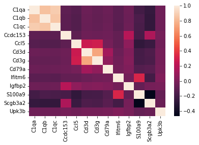
The estimated co-expression correlation matrix between genes can be vizualised as folow
[11]:
import seaborn as sns
from matplotlib import pyplot as plt
corr_matrix = []

for gene0 in  dataset.dict_co_expression:
    list_corr_gene0 = []
    for gene1 in dataset.dict_co_expression:
        list_corr_gene0.append(dataset.dict_co_expression[gene0][gene1])
    corr_matrix.append(list_corr_gene0)
list_gene = list(dataset.dict_co_expression.keys())
#plotting the heatmap for correlation
ax = sns.heatmap(corr_matrix, xticklabels = list_gene, yticklabels = list_gene,)
plt.show()
2) Create a graph of RNA molecule nodes and apply graph patitioning
we will use the previously computed co-expression matrix to weigth the KNN of graph of RNA
We will then partition this K-Nearest Neighbors (KNN) graph, into distinct communities of RNA molecules. These identified RNA communities are expected to group together neighboring RNA molecules that originate from co-expressed genes, and therefore, are likely to be from the same cell.
[12]:
import comseg
from comseg import model
from comseg import dictionary
[13]:
Comsegdict = dictionary.ComSegDict(
                 dataset=dataset,
                 mean_cell_diameter= MEAN_CELL_DIAMETER,
                 community_detection="with_prior",
)


Comsegdict.compute_community_vector()
0%| | 0/2 [00:00<?, ?it/s]
improvement of modularity 0.5175425675718313
improvement of modularity 0.1306392271844058
improvement of modularity 0.02507302657082544
improvement of modularity 0.0029234395689082815
50%|█████ | 1/2 [00:07<00:07, 7.41s/it]
improvement of modularity 0.5100496018417177
improvement of modularity 0.12578317556317042
improvement of modularity 0.03023102645415554
improvement of modularity 0.0034015267990896714
100%|██████████| 2/2 [00:13<00:00, 6.61s/it]
3) In situ clustering
[14]:
Comsegdict.compute_insitu_clustering(
                                  size_commu_min=3,
                                  norm_vector=True,
                                  ### parameter clustering
                                  n_pcs=3,
                                  n_comps=3,
                                  clustering_method="leiden",
                                  n_neighbors=20,
                                  resolution=1,
                                  n_clusters_kmeans=4,
                                  palette=None,
                                  nb_min_cluster=0,
                                  min_merge_correlation=0.8,
                                  )
/home/tom/.local/lib/python3.8/site-packages/anndata/_core/anndata.py:1838: UserWarning: Observation names are not unique. To make them unique, call `.obs_names_make_unique`.
  utils.warn_names_duplicates("obs")
Writing temporary files...
Running scTransform via Rscript...

Attaching package: arrow

The following objects are masked from package:feather:

    read_feather, write_feather

The following object is masked from package:utils:

    timestamp

Calculating cell attributes from input UMI matrix: log_umi
Variance stabilizing transformation of count matrix of size 13 by 486
Model formula is y ~ log_umi
Get Negative Binomial regression parameters per gene
Using 13 genes, 486 cells
  |======================================================================| 100%
Second step: Get residuals using fitted parameters for 13 genes
  |=================================================================           =====| 100%
Calculating gene attributes
Wall clock passed: Time difference of 0.2426596 secs
Reading output files...
Clipping residuals...
number of cluster 7
number of cluster after merging 8
[14]:
AnnData object with n_obs × n_vars = 639 × 13
    obs: 'list_coord', 'node_index', 'prior', 'index_commu', 'nb_rna', 'img_name', 'leiden', 'leiden_merged'
Next, we will create a UMAP visualization of the RNA profiles within each community. Specifically, each RNA community is linked to an expression vector. We then cluster these community expression vectors in a similar manner to how we would cluster single-cell RNA sequencing (scRNAseq) data. In the following UMAP, each dot corresponds to one RNA community.
[15]:
import scanpy as sc
import random
palette = {}
for i in range(-1, 500):
    palette[str(i)] = "#" + "%06x" % random.randint(0, 0xFFFFFF)
adata = Comsegdict.in_situ_clustering.anndata_cluster
adata.obs["leiden_merged"] = adata.obs["leiden_merged"].astype(str)
sc.tl.umap(adata)
fig_ledien = sc.pl.umap(adata, color=["leiden_merged"], palette=palette, legend_loc='on data',
                )
/home/tom/.local/lib/python3.8/site-packages/scanpy/plotting/_tools/scatterplots.py:394: UserWarning: No data for colormapping provided via 'c'. Parameters 'cmap' will be ignored
  cax = scatter(

[16]:
Comsegdict.add_cluster_id_to_graph(clustering_method = "leiden_merged")
100%|██████████| 11410/11410 [00:00<00:00, 304389.36it/s]
100%|██████████| 9632/9632 [00:00<00:00, 326973.49it/s]
[16]:
"ComSegDict {'07_CtrlNI_Pdgfra-Cy3_Serpine1-Cy5_004': <comseg.model.ComSegGraph object at 0x7f4b60b42790>, '07_CtrlNI_Pdgfra-Cy3_Serpine1-Cy5_006': <comseg.model.ComSegGraph object at 0x7f4b304122e0>}"
[17]:
from comseg.utils import plot
importlib.reload(plot)
img_name = list(Comsegdict.keys())[1]
G = Comsegdict[img_name].G
nuclei = tifffile.imread(
    your_path_to_test_data + f'/mask/{img_name}.tiff')


fig, ax = plot.plot_result(G=G,
            nuclei = nuclei,
               key_node = 'gene',
                dico_cell_color = None,
                figsize=(10, 10),
                spots_size = 10,
                title  = "ONE COLOR = ONE GENE")

fig, ax = plot.plot_result(G=G,
            nuclei = nuclei,
               key_node = 'leiden_merged',
                dico_cell_color = palette,
                figsize=(10, 10),
                spots_size = 10,
                title  = "ONE COLOR = ONE TRANSCRIPTOMIC CLUSTER")


4) final RNA-nuclei association
[18]:
Comsegdict.classify_centroid(
          n_neighbors=15,
          dict_in_pixel=True,
          max_dist_centroid=None,
          key_pred="leiden_merged",
          distance="ngb_distance_weights",
                        )
100%|██████████| 2/2 [00:00<00:00, 11.32it/s]
We now utilize the Dijkstra’s algorithm to link each nucleus centroid to the closest RNAs that are labeled with the same transcriptomic cluster.
[19]:
Comsegdict.associate_rna2landmark(
                         key_pred = "leiden_merged",
                         distance='distance',
                         max_cell_radius=MAX_CELL_RADIUS)
0%| | 0/2 [00:00<?, ?it/s]
07_CtrlNI_Pdgfra-Cy3_Serpine1-Cy5_004
100%|██████████| 10266/10266 [00:00<00:00, 497219.65it/s]
 50%|█████     | 1/2 [00:02<00:02,  2.21s/it]
07_CtrlNI_Pdgfra-Cy3_Serpine1-Cy5_006
100%|██████████| 8675/8675 [00:00<00:00, 455189.68it/s]
100%|██████████| 2/2 [00:04<00:00,  2.37s/it]
[20]:
importlib.reload(comseg)
from comseg.utils import plot
importlib.reload(plot)

G = Comsegdict[img_name].G
nuclei = tifffile.imread(
    your_path_to_test_data + f'/mask/{img_name}.tiff')

plot.plot_result(G=G,
            nuclei = nuclei,
               key_node = 'cell_index_pred',
                title = None,
                dico_cell_color = None,
                figsize=(15, 15),
                spots_size = 10,
                plot_outlier = False)
[20]:
(<Figure size 1080x1080 with 1 Axes>,
 <Axes: title={'center': 'cell_index_pred'}>)

the final output of this pipeline is an AnnData object so our model can be integrated into Scanpy/Scverse single cell workflow analysis. It contains for each cell an exppression vector, the cell centroid coordinates and the molecule coordinates associated to this cell.
[21]:
anndata ,jsons = Comsegdict.anndata_from_comseg_result(
                        return_polygon = False,
                        alpha = 0.6,
                        min_rna_per_cell = 5)
100%|██████████| 2/2 [00:00<00:00, 21.63it/s]
[22]:
Comsegdict.final_anndata.uns['df_spots']['07_CtrlNI_Pdgfra-Cy3_Serpine1-Cy5_006'].head(5)
[22]:
| node_index | x | y | z | gene | cell | cell_type | in_nucleus | nb_mol | index_commu | leiden_merged | cell_index_pred | distance2centroid | |
|---|---|---|---|---|---|---|---|---|---|---|---|---|---|
| 0 | 0 | 945 | 436 | 13 | C1qa | 8 | T_cells | 0 | 1 | 0 | 4 | 0 | inf |
| 1 | 1 | 1187 | 354 | 50 | C1qa | 8 | T_cells | 0 | 1 | 1 | -1 | 0 | inf |
| 2 | 2 | 1109 | 348 | 8 | C1qa | 8 | T_cells | 0 | 1 | 2 | 4 | 0 | inf |
| 3 | 3 | 644 | 528 | 18 | C1qa | 107 | Club | 0 | 1 | 3 | 4 | 0 | inf |
| 4 | 4 | 668 | 659 | 45 | C1qa | 107 | Club | 0 | 1 | 4 | 4 | 0 | inf |
[23]:
adata = Comsegdict.final_anndata
#sc.tl.pca(adata, svd_solver='arpack', n_comps = 0)
sc.pp.neighbors(adata, n_neighbors=30, n_pcs=0)
sc.tl.leiden(adata,  resolution=1)
sc.tl.umap(adata)
sc.pl.umap(adata, color=["leiden"], palette=palette, legend_loc='on data')
/home/tom/.local/lib/python3.8/site-packages/scanpy/plotting/_tools/scatterplots.py:394: UserWarning: No data for colormapping provided via 'c'. Parameters 'cmap' will be ignored
  cax = scatter(

[24]:
from pathlib import Path
anndata.write_h5ad( Path(your_path_to_test_data) / "result.h5ad")
[25]:
sc.read_h5ad(Path(your_path_to_test_data) / "result.h5ad")
[25]:
AnnData object with n_obs × n_vars = 75 × 13
    obs: 'CellID', 'Name', 'centroid_z', 'centroid_y', 'centroid_x', 'image_name', 'leiden'
    var: 'features'
    uns: 'df_spots', 'leiden', 'leiden_colors', 'neighbors', 'umap'
    obsm: 'X_umap'
    obsp: 'connectivities', 'distances'
[23]:
[ ]: